Beam position methods
This page describes how finding beam position works in DIALS (with the command
dials.search_beam_position). The methods described here are also used in
AutoED. Four methods are implemented in dials.search_beam_position
function: default, maximum, midpoint, and inversion method.
The default method is based on the work of Sauter et al. (please see Ref.
[1]) and it is not covered here. The other three methods are based
on projecting diffraction images, described below.
The three projection methods are designed primarily for electron diffraction images collected at eBIC, although nothing prevents you from using them for other sources. They work mainly in cases when the user can quickly determine the beam center just by looking at a diffraction image, and they do not rely on some profound mathematical truth. In other words, they are not a ‘silver bullet’ to handle every dataset, but an ad hoc solution that works for most datasets obtained at eBIC. The initial idea was to use the output of these methods to train a machine learning model (with problematic datasets labeled by hand).
It is unlikely that any of the three methods presented here will work on your data out of the box. Depending on the setup of your experiment, detector resolution, position of the beam stop etc, you will have to tune method parameters to fit your experiment. However, once you find the correct combination of parameters, the methods will work well for most of your datasets.
By default, all three methods work on the average diffraction image in a
dataset. For example, suppose you perform a rotational scan with a thousand
frames in a dataset. In that case, the methods will first extract each frame
separately, add those frames together, and compute the average image
representing that dataset. This can be time-consuming and sometimes
unnecessary, as beam position can be calculated based on just a few images
from a dataset. Therefore, all three methods provide options for data slicing
(similar to how slicing works in Numpy). See more about selecting image ranges
below. Another option is to compute beam position for each frame individually
instead of computing a single beam center for the entire dataset
(see more about option per_image=True below).
Maximum pixel intensity method
This is the simplest projection method, which is suitable for datasets where
the beam is visible (not occluded by a beam stop). Assuming we already
imported our dataset with dials.import, we can run the
search_beam_position on the imported experiment file
dials.search_beam_position method=maximum imported.expt
The output should be a single PNG image called beam_position.png
(see Fig. 2).

Fig. 2 Beam position computed using the maximum pixel intensity method. Data provided by Peter Ercius from Lawrence Berkeley National Laboratory.
The generated plot shows the average diffraction image in the central part and two projected profiles along the x- and the y-direction in the top and right panel, respectively. The beam position in pixels (rounded to an integer) is shown in the top-right corner. The plot has additional metadata, such as the image dimensions, the minimal and maximal pixel intensity, etc.
Note
By default, the plotting function will try to adjust the colormap range to
show high-intensity regions.
However, in some datasets, pixel intensities might be unevenly
distributed. Imagine a dataset where the average pixel has an intensity
between 0 and 10, but some bad pixels show intensities of several
millions. In that case, spotting the beam center on the average image
would be hard. If this is the case with your dataset, you can use the
option color_cutoff to lower the upper colormap limit. For example, in
Fig. 2, this option is set to color_cutoff=80 (see the
colormap range maximum in Fig. 2). Setting this parameter
will not change the original data; it will only change its coloring on the
graph. Pixels with intensities above the color cutoff would be set to the
same color. The color_cutoff also applies to other methods
(inversion and midpoint).
When projecting data from a 2D image to 1D profiles, we can either compute the average pixel intensity along an axis or find the maximal pixel along an axis. The previous figure shows both maximal and average projections (the grey and green curves in Fig. 2, respectively).
Because the beam is visible, one can find the pixel with maximum intensity and declare that to be the beam center without any projecting. However, this is not always correct. In some cases, bad pixels will return the maximal intensity from the trusted range by default. Also, there might be cases where the intensity of a reflection spot is higher than the intensity at the direct beam. One condition usually satisfied when the beam is visible is that the direct beam has the most extensive spread compared to other diffraction spots. Finding the broadest peak is a good starting point for computing the beam position. The next step is determining the pixel with the highest intensity within that broadest peak. Projecting the diffraction image along the x and the y is not necessary. However, it dramatically simplifies the problem by reducing it to one dimension. The downside is that there might be cases where strong reflection spot masks the direct beam in the projected profile. Averaging over few images (as in our example above) usually removes this problem.
The first step in the maximum method is to find the broadest peak
in a projected profile. This is done by scanning the average
projected profile (the green curves in Fig. 2) with an averaging
kernel of a certain width (see Fig. 3).

Fig. 3 Parameters bin_width and bin_step of the maximum pixel intensity
method. The averaging kernel is represented with the gray rectangle that
scans the projected profile. The rectangle width (in pixels) sets the
width of the moving average window, and the window moves in steps of
bin_step (again, in pixels).
The averaging kernel (the dark gray rectangle in Fig. 3) sweeps over
the projected profile moving in discrete steps (determined by the bin_step
parameter). The kernel size is set with the bin_width parameter. At each
position during the sweep, the kernel computes the
integral sum of the average projected profile beneath the kernel (the
green area below the green curve in Fig. 3). After sweeping the
entire
profile and computing profile integrals, the maximum method determines the
kernel position where this integral has the maximal value. In general, this
will correspond to an area where most of the projected profile intensity is
located (the broadest peak). For a real-world example, see the gray shaded
areas
in projected profiles in Fig. 2. These are kernel positions
with maximal integral, and they indeed correspond to the broadest peak.
Depending on the
image dimensions, the beam characteristics, etc, the user will have to
fine-tune the bin_step and bin_width parameters to match the expected
spread of the direct beam for the given experimental setup. To ensure the
continuous sweep across the projected profile, DIALS assumes that bin_step
is always smaller than bin_width, otherwise it will throw an error.
The next step is to find the actual beam position. For this, we use the maximum projected profiles (the gray curves in Fig. 2). The method finds a maximal pixel within the previously determined broadest peak (the gray-shaded areas in the projected plots in Fig. 2).
Other options
The user can additionally smooth the average projected profile by changing the
maximum.convolution_width parameter, which sets the width of the
convolution smoothing window before the kernel sweep. Also, the user
can set all pixels above a certain intensity to zero in the average
diffraction image (that is, before projecting onto the x and y-axis).
This is done using maximum.bad_pixel_threshold parameter.
The image_ranges argument is used for slicing, like in the Numpy
library. Image ranges are selected using the Numpy
slice notation, that is, start:stop:step, where any of the three numbers
can be omitted. Multiple ranges can be separated by commas
(e.g., image_ranges=0:3,7:20:2,35,48) which also
allows for the selection of individual images. This feature becomes
particularly helpful for large datasets. Instead of waiting for thousands of
images in a dataset to average, it is much faster to select only a subset of
those images.
One can additionally use
imageset_ranges to select between different imagesets (if they are present
in a dataset).
Besides computing the average image and then making the projection,
the user can compute beam position for each image separately
using per_image=True parameter. This will produce a series of PNG images.
beam_position_imageset_00000_image_00000.png
beam_position_imageset_00000_image_00001.png
beam_position_imageset_00000_image_00002.png
beam_position_imageset_00000_image_00003.png
...
Each image will contain information about beam position. Additionally, if
per_image=True, DIALS will produce beam_positions.json file with
a list of computed beam positions
 [
     [
         0,
         0,
         294.0,
         261.0
     ],
     [
         1,
         0,
         296.0,
         261.0
     ],
     ...
]
Here, the first number in the four-element list is the imageset index,
the second is the image index, and the third and fourth are beam positions
along the x and y direction (in pixels).
The JSON file will have beam positions for all
images and imagesets selected using image_ranges and imageset_ranges.
The user should also distinguish between method-specific parameters
(such as bin_width and bin_step) and parameters such as per_image
and image_ranges, which also apply to other projection methods as well.
See dials.search_beam_position -h for more info on the function
interface. The parameters that apply to all three projection methods
are under the projection keyword. Most parameters specific to the
maximum method (and other projection methods) apply both to projections along
the x and the y axis.
Midpoint method
This method is suitable for datasets where direct beam is blocked by some obstacle. Fig. 4 presents one such dataset. A Singla detector consists of two panels, with a gap between them. It is common for electron beam to be positioned in this gap. Determining the beam position based on the maximum pixel intensity will not work because the beam is hidden.
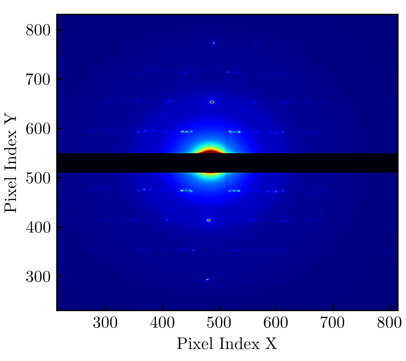
Fig. 4 A diffraction image from DECTRIS Singla detector at eBIC.
First, we run the midpoint method on this dataset without any parameters.
dials.search_beam_position method=midpoint imported.expt
The output of this command is shown below.
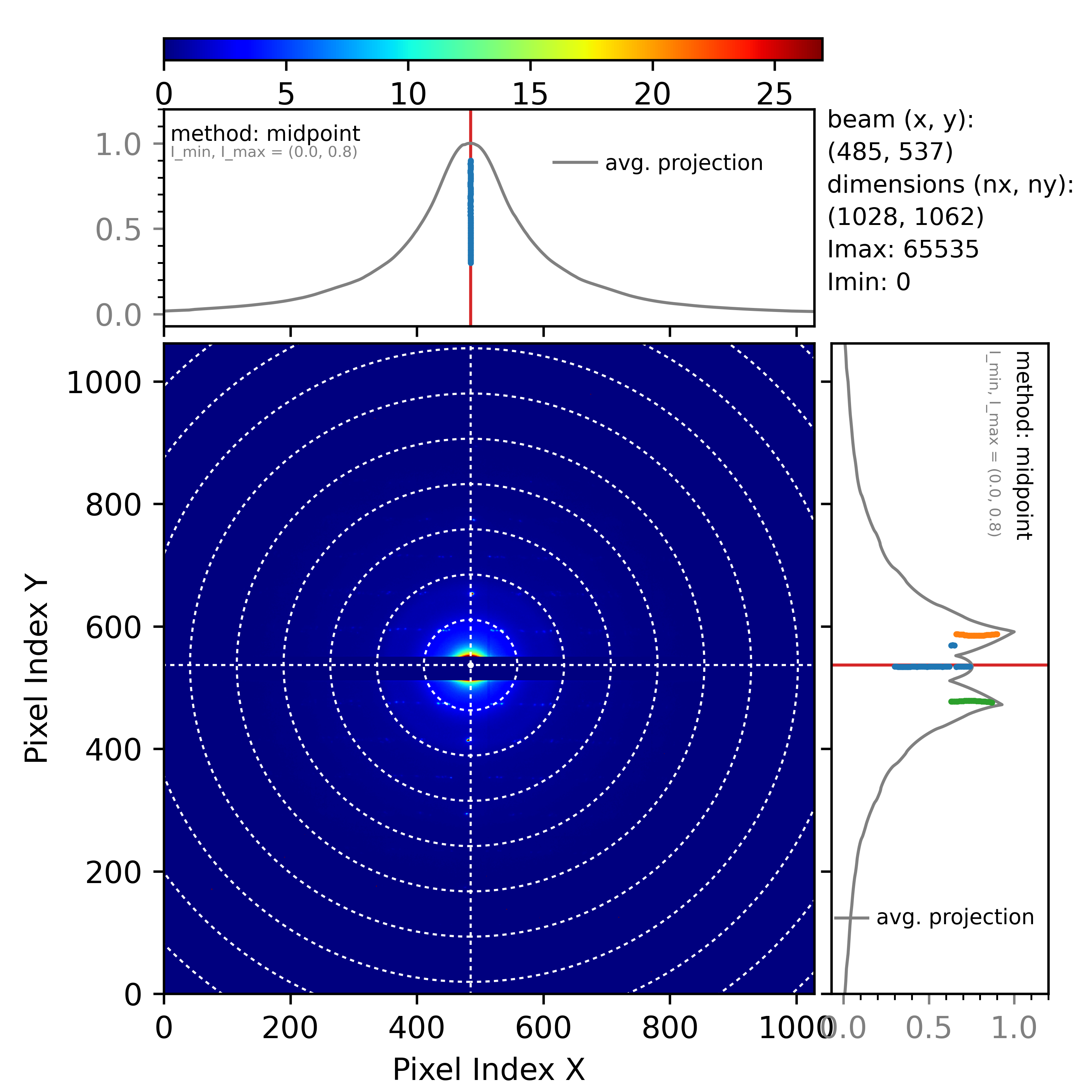
Fig. 5 Beam position determined by the midpoint method.
The midpoint method is similar to the maximum method in that the average pixel
intensity is projected. This projected intensity is then smoothed using a
convolution kernel (averaging intensities in a narrow window given by
midpoint.convolution_width). As with the maximum method, projecting bad
pixels will create unwanted peaks. To solve this, we
introduce a parameter exclude_intensity_percent. Before DIALS projects
a diffraction image, it will order all image pixels into a one-dimensional
array of increasing intensity. The exclude_intensity_percent tells DIALS
to discard the top percentage of these pixels (set them to zero). For
example, exclude_intensity_percent=0.1 will exclude 0.1 % of these
high-intensity pixels.
To further explain the midpoint method we can focus only on the projection
along the y axis.
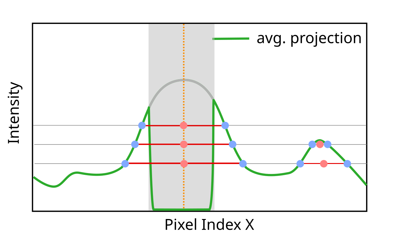
Fig. 6 How midpoint method determines the beam position. The green curve is the projected average pixel intensity, while the gray shaded rectangle marks the area where direct beam is blocked by some obstacle (the beam intensity in that region goes to zero).
Fig. 6 shows the projection profile’s appearance when some obstacle impedes the direct beam. The midpoint method will draw horizontal lines and compute the intersection points between these lines and the projected profile (the blue dots). Next, it will compute the midpoints between the intersections (the red dots). The average position of the calculated midpoints will correspond to the beam position (the orange vertical dashed line in Fig. 6).
The main assumption of the midpoint method is that the projected profile is
a reasonably symmetric function. If the profile is skewed, the position of the
average midpoint would not correspond to the beam position. The skewness might
come from hitting the detector at an angle. Fig. 5
shows a projected profile is normalized (put in the range between
zero and one). The number of lines intersecting the profile is set
with the intersection_range. For example, by default, the
intersection range is set from 0.3 to 0.9 with a step 0.01.
(intersection_range=0.3,0.9,0.01). With this setting, DIALS will draw
around sixty intersection lines. When using this parameter, keep in mind the
normalization, so always set it in the range between zero and one.
In Fig. 5 (the projection along the y-axis on the right), we
see several groups of midpoints (orange, blue, green). Each of these groups
corresponds to a local peak in the projected profile. As shown in
Fig. 6, each intersecting line might intersect several
peaks in the projected profile. The question is: which peak is the direct one?
Here, DIALS does several things. First, it groups all the midpoints into
distinctive groups based on their proximity. The grouping is determined using
the distance_threshold parameter (currently set to 40 pixels). The
condition for a new midpoint to be included in an existing group is if it is
within the distance_threshold of any known group (that is, the group
average position). If the midpoint is not close to any of the existing groups,
it will be added to a new group. Next, groups are ranked based on their
average width. The average width is computed by averaging the widths of all
the intersection lines belonging to a group (see the red horizontal lines in
Fig. 6). In the final step, DIALS picks the first three
groups of midpoints with the highest average width and selects the one with
the highest number of midpoints. This last step ensures that we do not pick a
group with only a few intersections (in most cases, the direct beam will have
the highest width and number of midpoints). The beam position is then
computed as the average midpoint position of the selected group.
Dealing with gap regions
By default, DIALS does not know which region of the image corresponds to the gap. For example, in the case of the Singla detector, all pixels from 512 to 550 along the y-axis are in this gap region. Our result along the y-axis in Fig. 5 was correct, but it was more a lucky coincidence. The wide convolution of the projected profile filled the gap and allowed the midpoint method to work as expected. However, if the convolution width was too narrow (or the gap was too wide), the midpoint method would not work as expected. To explain what we mean, let’s run the same command, but let’s not smooth the projected data.
dials.search_beam_position method=midpoint \
                           midpoint.convolution_width=2 imported.expt
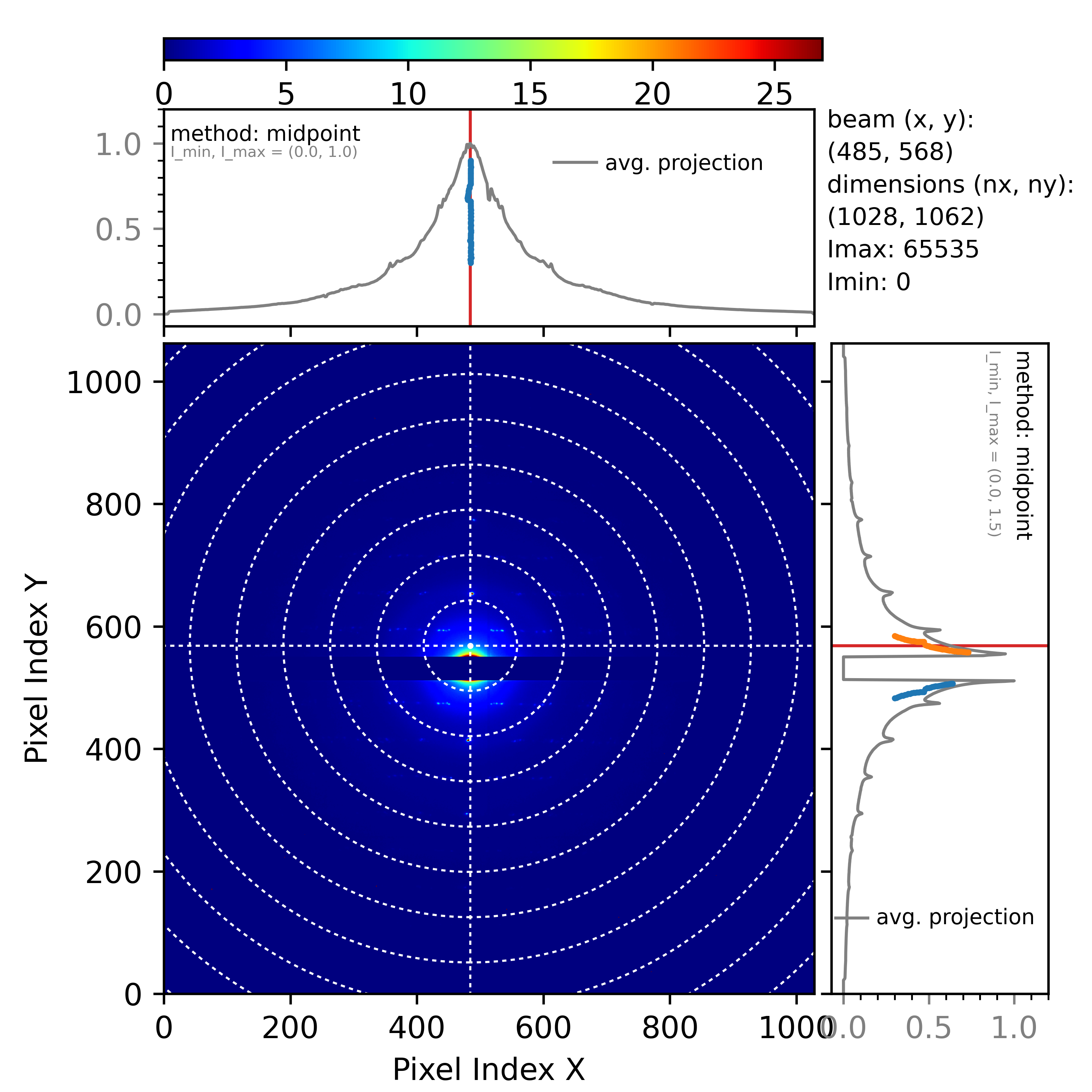
Fig. 7 Result from the midpoint method obtained with the command above.
Fig. 7 shows the wrong beam position along the y-axis. The reason for this error is simple to explain. Without any convolution, the projected gap region gets an intensity of zero. The problem here is that DIALS does not know where the gap is. It treats the two beam tails as two separate peaks (that is why there are two groups of midpoints, the orange and the blue). To resolve this problem, we need to tell DIALS where the gap is.
dials.search_beam_position method=midpoint \
                           midpoint.convolution_width=2 \
                           dead_pixel_range_y=505,555 imported.expt
This will produce the correct result
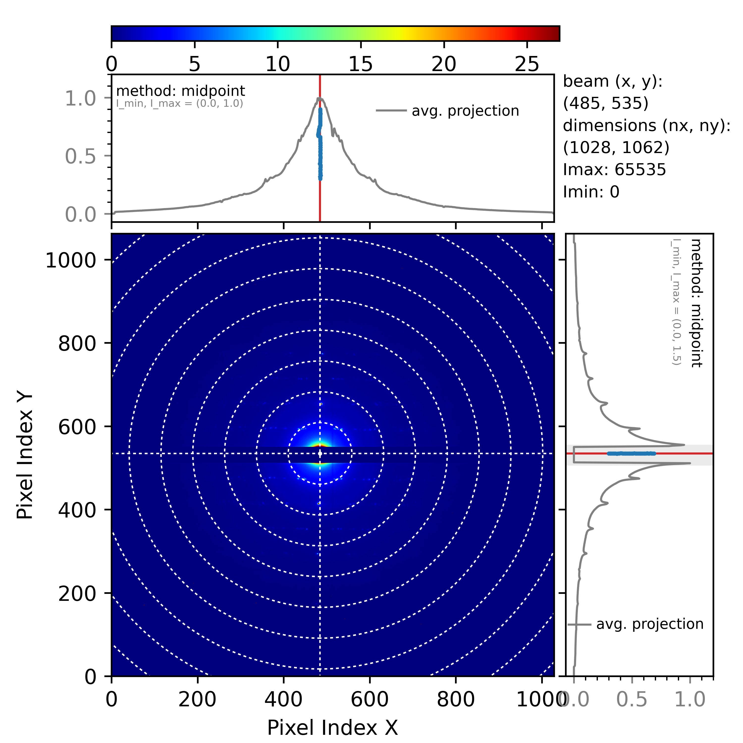
Fig. 8 Beam position corrected with dead_pixel_range_y parameter.
Notice that the dead pixel range along the y-axis that we provided as a
parameter is marked with the gray shaded rectangle in the y-projected
profile in Fig. 8. Also, we set the region of dead pixels to
be slightly wider than the actual gap region (by about five pixels on both sides).
The simple explanation of the dead_pixel_range_y is that DIALS will ignore
all intersections within this region. This is equivalent to filling the gap
region with infinite intensity. The intersections with the two tails of the
original beam are now accounted for properly, and the midpoint method works
again.
Equivalently to dead_pixel_range_y, there is a parameter
dead_pixel_range_x. Additionally, you can use multiple ranges like
dead_pixel_range_y=a,b,c,d. This will set two regions (from a to
b, and from c to d).
Inversion method
This method is suitable for datasets where one can clearly see Friedel pairs.
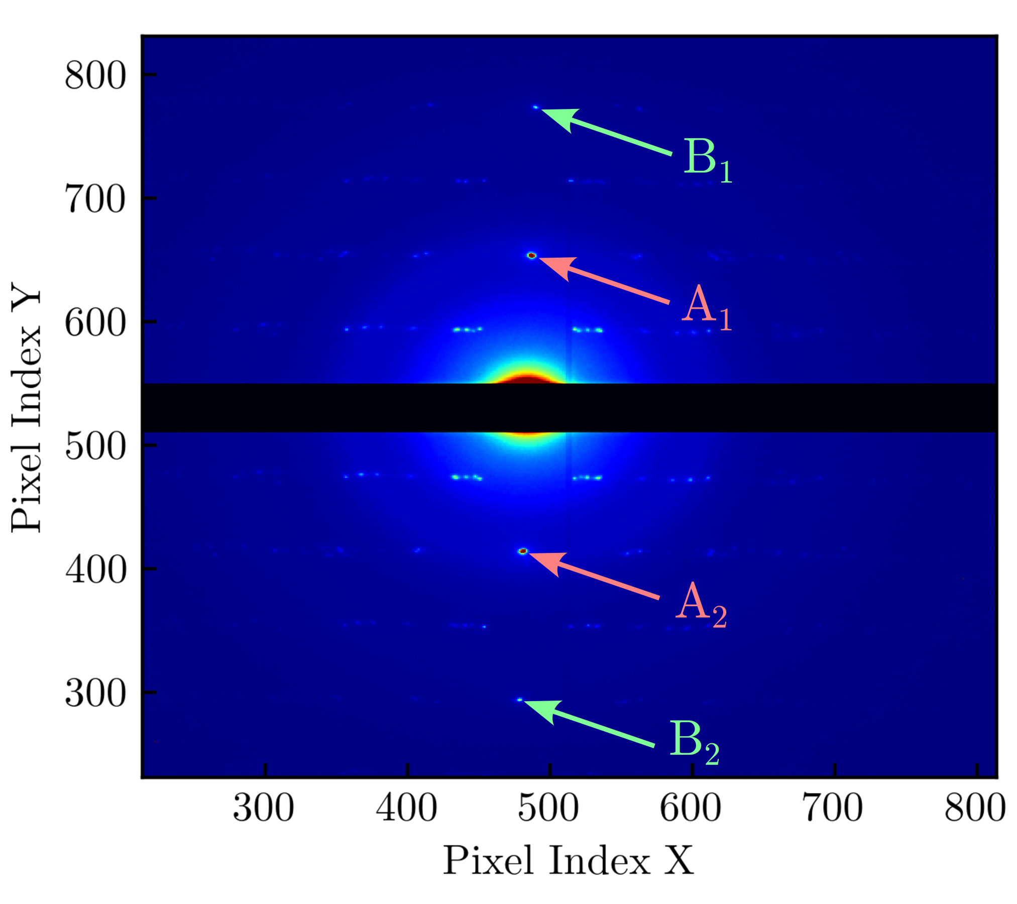
Fig. 9 Friedel pairs (A1, A2) and (B1, B2) in the Singla diffraction image obtained at eBIC.

Fig. 10 Sketch of the projected profile with Friedel pairs (no direct beam).
For example, Fig. 9 shows the previous diffraction image from Singla, emphasizing two Friedel pairs. Friedel pairs are positioned symmetrically around the direct beam. In this case, the simplest way to determine the beam position is to connect a single Friedel pair with a vector and divide that vector in half. Another approach would be spot-finding first to determine the positions of Friedel pairs and then compute the midpoints. We plan to use projection again to simplify the problem. To explain the inversion method, let us assume we make maximum projection along the y-axis from Fig. 9, and we obtain something similar to the sketch in Fig. 10. There are four peaks corresponding to two Friedel pairs. Because of the equal distance from the direct beam to both spots in every Friedel pair, the beam position becomes the center of inversion. The question is how to find this point for four peaks in Fig. 10 automatically. One can connect the peaks with lines, compute midpoints, and average them, but which peaks should be connected?
In our approach, we use a simple observation. Let us
assume the direct beam is positioned at some point called guess_position
(see Fig. 10). We can then invert the projected profile
around this point and obtain the pink curve. If guess_position is indeed
the center of inversion, the peaks in the inverted curve and those in the
original curve will overlap. If this is not the case, the peaks from one curve
will overlap with some other peaks (with different intensities) or with
low-intensity regions. One way to quantify the overlap between the original
and the inverted curve is to multiply them for each pixel and integrate (sum)
the product. If the overlap is significant, the integral will be large; if the
overlap is low, the integral should be lower. We repeat this procedure
(invert and compute the overlap) in a region around the guess_position.
We move the guess_position
to every point within this region, multiply the two curves, and compute the
integral to quantify the overlap. Ultimately, we will get a single curve that
quantifies the overlap for a range of pixels. Picking the maximum of this
curve as the beam position means that the computed overlap at that point is
highest, so that point is very likely to be the center of inversion.
We can check how this is implemented in DIAL by running the beam position command.
dials.search_beam_position method=inversion imported.expt
Below is the output of this command. The green curves in the top and right panels show the overlap (inversion and integration) for every pixel.

Fig. 11 The output of the beam position command with the inversion method.
The inversion method works well if there is at least one dominant Friedel pair. As shown in Fig. 11, there are several such peaks for an average image in a dataset.
[1] Sauter et al., J.Appl.Cryst. 37, 399-409 (2004).